Ariel University
Course name: Deep learning and natural language processing
Course number: 7061510-1
Lecturer: Dr. Amos Azaria
Edited by: Moshe Hanukoglu
Date: First Semester 2018-2019
Recurrent Neural Networks (RNN)
Introduction
An analysis of sentences is used in many fields, such as translating one language into another, writing a description of pictures, analysis of sound, etc. In order for us to perform the task properly and we can understand and create new sentences we must understand the content of the entire text and not just check what words appear in it.
In this tutorial we will focus on the analysis of text by Recurrent Neural Networks (RNN).
On the face of it, we can ask why not use a fully-connected network to analyze the trial?
In order to use fully-connected we will need to convert the sentence into a form that we can insert into the network.
One method is a bag of words. This method is not a good method because in this method we do not give importance to the order of the words within the sentence, and the order of the words in the sentence is very critical for proper understanding of the meaning of the sentence.
For example:
- The child ate pizza and did not eat vegetables
- The child ate vegetables and did not eat pizza
The meaning of these two sentences is the opposite of each other, but if we implement the bag of words method for both sentences we will get the same result.
Therefore we can not use this method.
And the use of the one hot method to represent the words, which gives importance to the location of the words in the sentence, is incorrect because then we do not give importance to the meaning of the words but give all the words the same weight.
Another way to try is to use CNN, since CNN gives importance to information points that are close to each other. But still do not receive general evidence of the entire trial.
Therefore, as noted above, we will learn a new method for analyzing text called RNN.
As we mentioned above, analysis of text can be in many cases. We will detail these cases:
- One to one - The input is single (single image or word) that is classified into a single class (binary classification). For example: Is it home or not?
- One to many - The input is single (image) that is categorized into many departments or written (in words) to the image. For example: for this image
 credit
We want it to say: Two birds fly. many to one - The input is a group (images or words) that is classified into a single class (binary classification). For example: Does the video (group of pictures) show a birthday party or not, is the sentence urgent or not.
Many-to-Many Input is a group (images or words) that is converted to another group.
- Translation of sentences. The text is first decoded and only then is the answer given to the output.
- Automatic speech recognition. Speech is deciphered directly into text, you hear a word and translate it and then another word and translate it too.
Description of the network structure
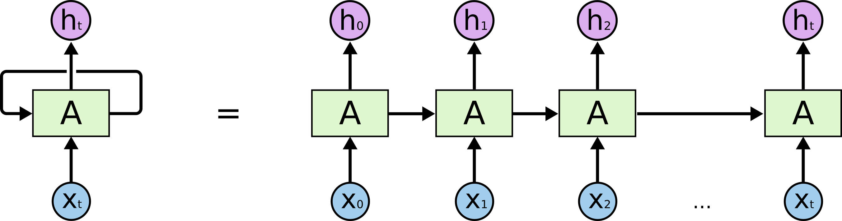
The RNN structure is: In each iteration get the next character / word $(x_i)$ and the memory of all the so-called until now. The output is the next character / word or the translation / meaning $(h_i)$ of the text so far, the output is also input to the next iteration.
Each of the iterations is represented by a square that is written inside it.
The two structures are identical, but the right structure is the non-rolled form of the left structure.
After we have seen the general structure of all iterations, we will now focus on the internal structure of each iterations.
After we have seen the general structure of all iterations, we will now focus on the internal structure of each iterations.
RNN has several different implementations
- Long Short Term Memory (LSTM)
- GRU
We will explain the implementation of each method.
Long Short Term Memory (LSTM)
The full appearance of the internal structure of each iteration is
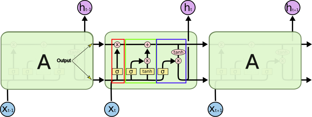
Now we will explain each and every part of the above structure:
- The red part: Forget what has been learned until now. That is, doubling the "memory" in the number from 0 to 1 when 0 means forgetting everything learned until now and 1 means remembering everything that has been learned until now, each number in this range means a few percent to remember from what has been learned so far. The sign $\sigma$ symbolizes logistic regression. The input is the previous memory and the new word (which is not yet read) and the output is a number between 0 and 1 as described above.
- Green part: remember the new thing learned (in addition to the old memory) and if so, how much of it to remember, that is, what importance to give to the new thing. That is, this part is responsible for adding memory to the long-term memory.
This section consists of two parts:
- Logistic regression that determines whether to remember the new thing. His input is the old memory and the new word and his output is a number between 0 and 1 that says whether to remember.
- Creates the new memory and adds it to the old memory.
- Blue part: says how much of all memory created at this stage should move on. We put the memory into the tanh function to get numbers between -1 and 1. The result will be the input of the next step. That is, this part is responsible for short-term memory, the memory that goes to the next stage.
In order to expand your understanding of the subject you can read on this web is a great web that explains the entire structure very well.
How Many Weights In LSTM?
One of the important parameters in understanding the system structure is knowing how many weights there are in the system.
To do this we will perform an analysis of the amount of weights in the system.
Let's mark a few things:
- k - The dimension of the new input $(x_i)$
- d - the dimension of the memory transferred from one stage to another (the width of the horizontal lines)
- t - like steps / cells
- m - Mini-batch size
In this implementation, we perform 3 times linear regression and one time tanh, each function is performed d times (for each memory cell). For each of the functions the inputs are entered, $x_i$ (k weights) and the memory from the previous step (d weights), that is there are k + d weights and d d times.
So the total account is: $\left(\left(k + d\right) + 1 \right) * 4 * d$
It can be seen that m and t do not affect the number at all.
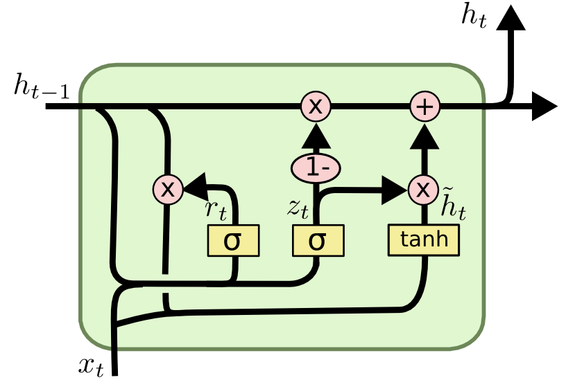
GRU
A different method for realizing RNN is called GRU. The realization of this method is shown in the image below. This method is similar in its parts to the previous method (LSTM) but has joined several parts together.
Generating Text in TensorFlow With RNN
import tensorflow as tf
import numpy as np
import urllib
#A list that holds all characters as ASCII values
all_text = [ord(x) for x in list(urllib.request.urlopen("https://s3.amazonaws.com/text-datasets/nietzsche.txt").read().decode("utf-8"))]
batch_size = 15
num_past_characters = 10 # The number of previous characters that predict the next character
step = 1
# A list that holds "representative" for each ASCII value in the text,
# that is, if there are ASCII values in the text: 65,65,81,70,81 then this list will hold 65,81,70
char_mapping = list(set(all_text))max_char = max(char_mapping)
possible_chars = len(char_mapping) #The number of different possible text characters
inverse_char_map = np.zeros(max_char+1, dtype=int)
for i in range(possible_chars):
inverse_char_map[char_mapping[i]] = i
num_input_examples = int((len(all_text)-(num_past_characters+1))/step)
curr_batch = 0
Create data for the train.
In data_x there are $|batch\_size|$ rows in each of them have $|num\_past\_characters|$ characters and each character is represented by the one hot method, meaning that each character is represented by an array of the size of $|possible\_chars|$
In data_y there are the characters that each of the sentences should predict, which means that each sentence has one character represented in the one hot method, so the size of data_y is $|batch\_size|$ rows and $|possible\_chars|$ columns.
def next_batch():
global curr_batch
curr_range_start = curr_batch*batch_size
if curr_range_start + batch_size >= num_input_examples:
    return (None, None)
data_x = np.zeros(shape=(batch_size,num_past_characters,possible_chars))
data_y = np.zeros(shape=(batch_size,possible_chars))
for ep in range(batch_size):
    for inc in range(num_past_characters):
data_x[ep][inc][inverse_char_map[all_text[curr_range_start+ep*step+inc]]] = 1
    data_y[ep][inverse_char_map[all_text[curr_range_start+ep*step+num_past_characters]]] = 1
curr_batch += 1
return (data_x, data_y)def back_to_text(to_convert): # gets a one-hot encoded matrix and returns text. We'll need this at the end
return [chr(char_mapping[np.argmax(letter)]) for letter in to_convert]
a = next_batch()
a[0].shape
a[1].shape
np.max(a[0])
np.max(a[0],2)
np.argmax(a[0],2)
cellsize = 30
x = tf.placeholder(tf.float32, [None, num_past_characters, possible_chars])
y = tf.placeholder(tf.float32, [None, possible_chars])lstm_cell = tf.nn.rnn_cell.BasicLSTMCell(cellsize, forget_bias=0.0)
output, _ = tf.nn.dynamic_rnn(lstm_cell, x, dtype=tf.float32)output = tf.transpose(output, [1, 0, 2])
last = output[-1]W = tf.Variable(tf.truncated_normal([cellsize, possible_chars], stddev=0.1))
b = tf.Variable(tf.constant(0.1, shape=[possible_chars]))z = tf.matmul(last, W) + b
res = tf.nn.softmax(z)cross_entropy = tf.reduce_mean(-tf.reduce_sum(y * tf.log(res), reduction_indices=[1]))
train_step = tf.train.GradientDescentOptimizer(0.1).minimize(cross_entropy)
sess = tf.InteractiveSession()
sess.run(tf.global_variables_initializer())correct_prediction = tf.equal(tf.argmax(y,1), tf.argmax(res,1))
accuracy = tf.reduce_mean(tf.cast(correct_prediction, tf.float32))num_of_epochs = 200
for ephoch in range(num_of_epochs):
acc = 0
curr_batch = 0
while True:
    batch_xs, batch_ys = next_batch()
    if batch_xs is None:
break
    else:
sess.run(train_step, feed_dict={x: batch_xs, y: batch_ys})
acc += accuracy.eval(feed_dict={x: batch_xs, y: batch_ys})print("step %d, training accuracy %g"%(ephoch, acc/curr_batch))
def text2arr(source, start):
src_as_num = [ord(x) for x in source]
ret_arr = np.zeros(shape=(1,num_past_characters,possible_chars))
for inc in range(num_past_characters):
    ret_arr[0][inc][inverse_char_map[src_as_num[start+inc]]] = 1
return ret_arrrequested_length = 200
text = list("hello world")
for i in range(requested_length):
predicted_letter = back_to_text(res.eval(feed_dict={x:text2arr(text, len(text)-num_past_characters)}))
text += predicted_letter
print(''.join(text))
One of the problems caused by predicting text can be that you enter a loop and then the text is duplicated and does not produce new text but repeats existing text. This problem is created once the characters that guess the next character are repeated. In order to solve this problem, we will drag the following character according to the softmax returns, which means that a character with a high probability in softmax will be more likely to be the next character, in such a way that the probability of receiving a sequence of characters is the same as the previous ones.
tf.nn.rnn_cell
tf.nn.rnn_cell.BasicLSTMCell.__init__(num_units, forget_bias=1.0, state_is_tuple=True, activation=tanh)
Documentation of the function in this link
Multiple Layers of RNN
As we could take a single neuron and produce from it a grid with several layers so we can also produce a grid with several layers of RNN which means that all h_i will become x_i of the next layer.
The code that does this is:
cells_size = [120, 70, 50]def get_lstm_dropout(cellsize, dropout):
lstm_cell = tf.nn.rnn_cell.BasicLSTMCell(cellsize, forget_bias=1.0)
   dopoutRNN = tf.nn.rnn_cell.DropoutWrapper(lstm_cell , output_keep_prob=dropout)
return dropoutRNNrnn_cell.MultiRNNCell([get_lstm_dropout(mem_size, dropout) for mem_size in cells_size])
BLEU (Bilingual Evaluation Understudy) ScoreRNN
BLEU is a measure of the quality of translation carried out by machine translation (MT, candidates) in relation to the translation of a professional person (reference sentence), which takes into account the general translation and does not refer to lack of intelligence or grammatical errors in translation. This metric is based on a comparison of candidate for the correct translation of the sentence, reference sentence. The output is a number between 0 and 1 where as close to 1 means that it is closer to the reference sentence.
The algorithm:
- Divide the candidate into n-gram units (usually used in 4-gram).
- Sum the number of times each candidate n-gram unit appears in the reference sentence and divide the number of n-gram units in the candidate. (When one unit is checked, the order of the words is not important, but whether or not the words appear)
Because of the algorithm's method of operation, it will give a higher score to shorter sentences, whereas in many cases the long sentences are correct and therefore we will multiply the result given by the algorithm by $e^{1-r/c}$, r is the total length of all the reference sentences, c is the total length of all the candidates